Pound-Drever-Hall on an FPGA

May 15, 2026

This is a hardware/software co-design implementation of a Pound-Drever-Hall (PDH) laser frequency locking system on a Red Pitaya STEMlab 125-14 (Xilinx Zynq XC7Z010 SoC). Real-time signal processing runs on the FPGA (PL), a TCP control server runs on the ARM cores (PS), and a Python client API drives it all from a host machine. Before getting to the implementation, it’s worth building up why any of this is needed and how it actually works.

Why would you want this?

An ideal laser is a light source where the emitted field is perfectly coherent. In other words, if you sample the field at any two points in space or any two points in time, there’s a deterministic phase relationship between them. This doesn’t actually happen in practice. Various noise sources can introduce photons that are out of phase with the main field, and once those mix in, the aggregate phase of the beam starts doing something partially random. At that point the deterministic relationship breaks down and the beam is no longer coherent. This is a problem when the exact phase or frequency of the laser needs to be maintained. One example is gravitational wave detection, where the phase difference between two laser beams encodes spatial distortion from a passing wave. Another is optical communication using Phase-Shift Keying (PSK), where information is encoded in the relative phase of the carrier. And since frequency is just the first derivative of phase and wavelength follows from frequency, random phase noise also translates to wavelength jitter, which matters in applications like laser isotope separation, where the wavelength needs to sit on the absorption line of a specific isotope. There are a bunch of other examples but they won’t be covered here.

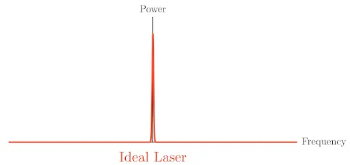
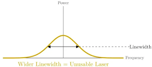
TL;DR: really clean lasers can be useful.

How PDH works

PDH locking extracts frequency-offset information from a laser relative to a stable reference (e.g. a cavity). The method works by phase-modulating the laser beam to generate sidebands, which can be described using the Bessel expansion of a modulated sinusoid. The cavity reflects the carrier and sidebands differently, encoding frequency detuning into a phase shift of the reflected light. By demodulating this signal at the modulation frequency, we recover an error signal that is directly sensitive to frequency offset.

Modulation and sidebands

The first thing we do is take a time-domain sinusoid and modulate it with an electro-optic modulator (EOM), which periodically phase-shifts the signal at some modulation frequency. If we look at the modulated signal we see something that seems similar to multiple sinusoids of different frequencies superimposing on each other:

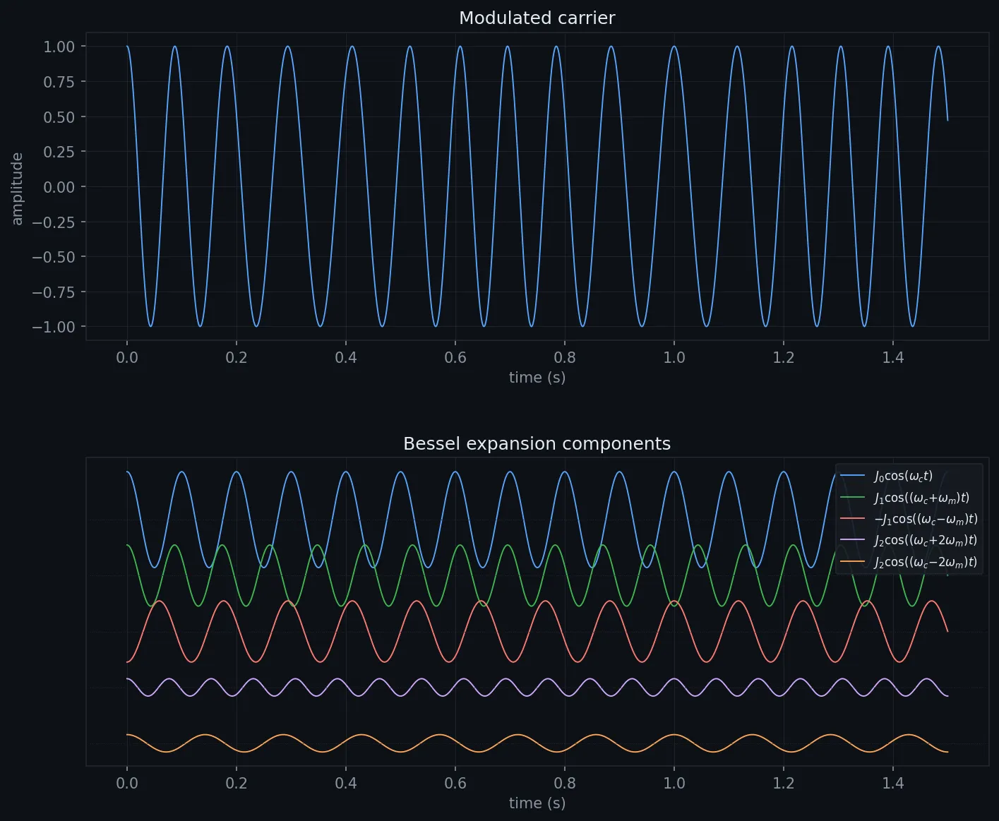
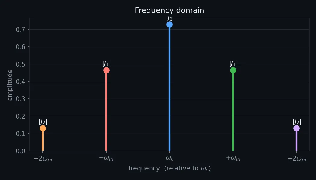
For modulation frequencies less than the carrier frequency, and for comparatively small values of the modulation depth $\beta$, we observe two prominent sidebands equidistant on each side of the carrier. A properly designed PDH system ensures the modulation frequency is much lower than the carrier and that $\beta$ is fairly small.

The reason this decomposition works is the Jacobi-Anger identity:

so our modulated sinusoid is

where

It’s relatively easy to see from the integral that for small $\beta$ and large $n$, the magnitude is quite low: integrating a high-frequency sinusoid across many cycles tends to yield a very small average. So for small $\beta$ we only really care about the first two terms, $J_0$ and $J_1$:

When $\beta$ is small the frequency spectrum shows three contributions: one large one at the carrier, and two smaller ones at the carrier $\pm$ the modulation frequency. These are the sidebands. Make $\beta$ larger and the higher Bessel terms start contributing, the spectrum sprouts more spikes, and we don’t want that, so we keep $\beta$ small.

The cavity

We now need something that imparts a phase shift on the carrier with respect to frequency drift that is (1) odd-symmetric, (2) as sharp as possible so we can detect it easily, and (3) centred on the carrier frequency we’re trying to lock to. We accomplish this with either a Fabry-Perot cavity or a ring resonator. For our purposes they’re functionally the same: they rotate the carrier with respect to frequency offset, and we demodulate the reflected field with respect to the modulation frequency.

Assuming a symmetric Fabry-Perot cavity with no losses, the reflection coefficient is

where $r$ is the amplitude reflection coefficient and $\Delta v_{fsr} = \frac{c}{2L}$ is the free spectral range (the spacing between modes) for a cavity of length $L$.

We can think of the reflection coefficient as a complex-valued vector whose phase depends on the carrier frequency. The reflected field is just the incident field stretched and rotated in the complex plane by this vector. Most of the time the vector is relatively real-valued and constant in magnitude. But approaching resonance it becomes almost entirely imaginary and flips across the real axis from $\pm i$ to $\mp i$, with magnitude going to zero at resonance. That sign flip is exactly the odd-symmetric response PDH exploits. For all other frequencies there’s little transformation beyond a $\pi$-phase flip, which is why the sidebands aren’t strongly affected by a well-designed cavity.

A ring resonator is a roundabout for light that accomplishes much the same thing as a Fabry-Perot cavity, but with a generally higher quality factor. Some of the incoming field couples into the ring, loops around, and interferes with the field that went straight through, and because each field also couples back out on the way around you get a convergent series. The full coupled-mode derivation is greasy algebra that ends at the same kind of transfer function:

Either way, the cavity encodes frequency offset into the phase of the reflected carrier, which is all we need.

The error signal

With the reflected field in hand we can write the reflected power. Dropping the DC terms and higher harmonics (they demodulate to zero against the base tone), the part we care about is

$F(\omega)$ and $F(\omega \pm \omega_m)$ are complex constants; we add their real and imaginary components tip-to-tail to get a resultant vector, and that vector rotates around the origin at $\omega_m$ via the $e^{i\omega_m t}$ term. At any instant the reflected power we observe is this vector’s projection onto the real axis, effectively a cosine wave at the modulation frequency whose amplitude is the resultant’s magnitude. Demodulate that tone with a phase mixer and pass it through a low-pass filter to recover the DC term, and that DC term is the error signal:

where $\phi$ is the mixer offset relative to the original modulating signal.

Imparting a phase shift on the modulator rotates the resultant vector $\gamma = F(\omega)F^*(\omega+\omega_m) - F^*(\omega)F(\omega-\omega_m)$, and the error signal is its projection onto the real axis. We want the projection to move as rapidly as possible outward in either direction as we detune from resonance, so we align $\gamma$ to lie along the real axis, in phase with the modulating tone, as much as possible across the detuning range. On the error-signal plot this corresponds to the modulation phase that produces the sharpest possible slope about resonance.

The toy error signal is odd-symmetric around resonance and monotonic in either direction up to a point. Past that point the derivative changes sign and the error signal is no longer reliable, which is why servo controllers are paired with a separate acquisition strategy (sweep-and-hold, or an auxiliary wide-range actuator) to get the laser close enough that the PDH slope is usable in the first place.

Orthogonal demodulation

In practice we extract the magnitude of that power phasor with an IQ mixer, independent of its phase offset relative to our IQ signals. The only random phase error we can’t account for in the RF design comes from the EOM’s residual amplitude modulation (RAM), which shows up as a phase shift on the photodiode output, and realistically that stays well under $\pm\frac{\pi}{3}$. So we square the LPF outputs of both mixer ports and add them to recover the squared magnitude of the phasor, then sign the result from the I-port output (positive if I is positive, negative otherwise). That gives a clean, phase-insensitive error signal.

TL;DR: beam → EOM → cavity → photodiode → demodulator. The sidebands carry the error signal; demodulating them recovers it, and from there we can generate a control signal to correct the laser.

Closing the loop

Having an error signal is only half the job; we still have to feed it back to the laser in a way that actually converges. I find it much more powerful and rewarding to think of control theory as a form of applied recursion than as a bag of block-diagram hacks implemented through black-box MATLAB code.

The open-loop transfer function is the product of all loop components, $\alpha = \hat{K}\hat{G}\hat{H}$. Using negative feedback, feeding the last output back to be subtracted from the input, the closed-loop response is

The recursion view makes this concrete. Let $h(t)$ be the open-loop impulse response. Expanding the loop pass by pass gives a Neumann series,

whose steady state maps cleanly to the Laplace domain:

The frequency-domain form is just the sum of the infinite series of convolutions describing the limiting behaviour of the feedback process. (There’s a more rigorous measure-theoretic way to define this so the series converges for the right conditions, but I don’t understand it, so enjoy the ghetto Neumann series instead.) Real systems also have a delay $\tau$ between input and output, which we fold in as a $\tau$-shifted delta convolution at each step; the closed loop becomes

and its stability is set by the roots of $1 + H(s)e^{-s\tau} = 0$.

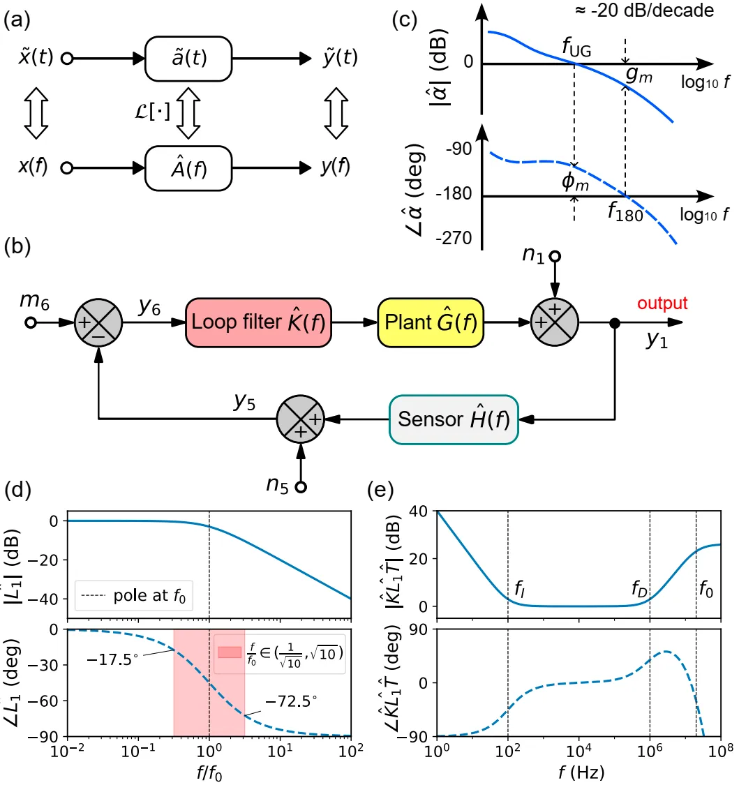
Working on the imaginary axis, we define unity gain as the frequency where the open-loop gain magnitude hits one ($|\alpha(f_{UG})| = 1 = 0\,\text{dB}$) and the phase margin as $\phi_m = \pi + \angle\alpha(f_{UG})$, how much room we have before $\angle\alpha = \pi$ at unity gain lands us on a pole. The error response $\frac{e}{x} = \frac{1}{1+\alpha}$ bumps up near unity gain, where $|1+\alpha|$ is smallest; this servo bump is the frequency at which the controller is worst at tracking disturbances, since modes there contribute disproportionately to the loop’s lifetime error.

The noise tradeoff

Modelling the loop’s sensitivity to the two noise sources separately, the laser (plant) noise $n_1$ and the sensor noise $n_5$ see

As we approach ideal negative feedback ($|\alpha| \to \infty$, $\angle\alpha = 0$), laser-noise sensitivity goes to zero while sensor-noise sensitivity approaches $-\frac{1}{H}$. So high gain at the frequencies of interest suppresses laser noise at the expense of injecting more sensor noise, which the loop can’t correct because it’s inside the measurement. That tradeoff, plant vs sensor noise, has to be weighed during design.

Laser noise itself is a mix of Gaussian white noise and flicker noise, with a PSD of the form

White noise is fundamentally just adding entropy: it washes out the structure of the Lorentzian line uniformly. Flicker noise, on the other hand, is a comically dressed villain who loudly proclaims “I will change your laser’s frequency for a relatively long period of time and mess up your frequency spectrum in the process.” It squeezes the sides of the line inward and makes the top more pointy, because small, long-lived frequency deviations are statistically more likely than large ones.

Tuning

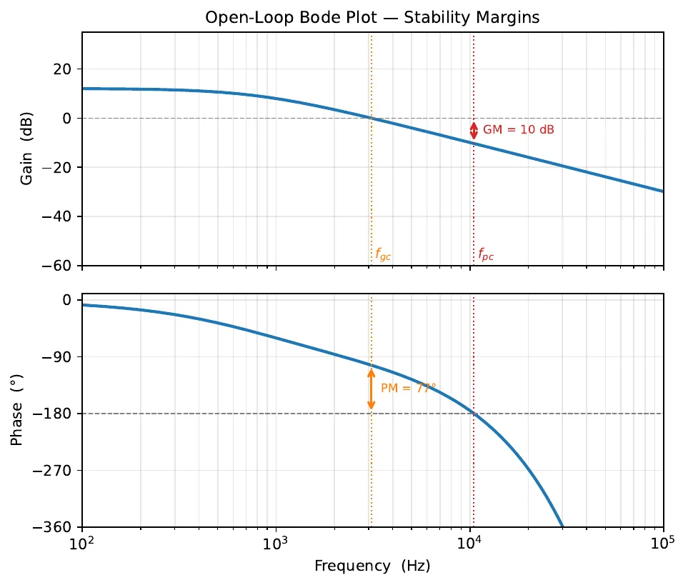
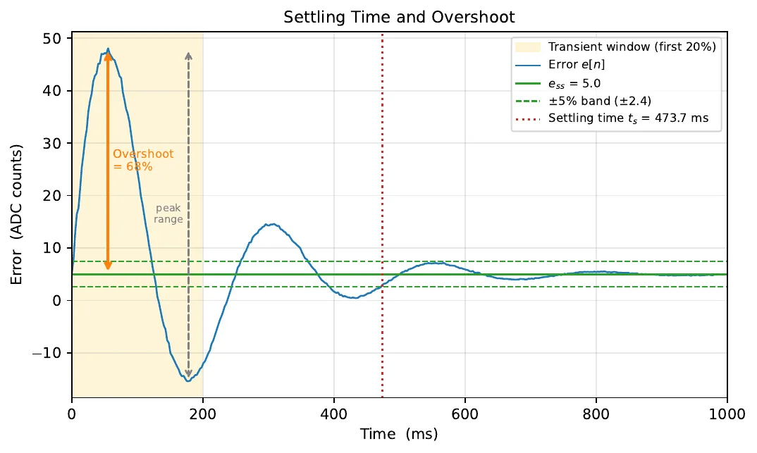
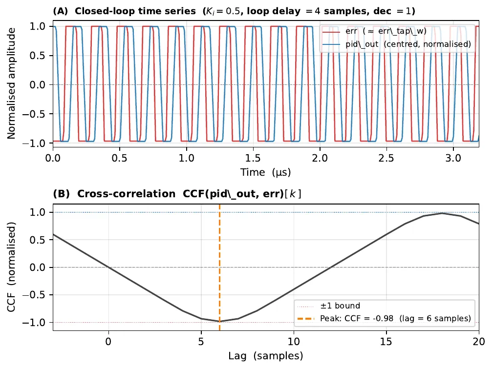
We generally optimize two of {performance, bandwidth, robustness} at the expense of the third, so it makes sense to fix a minimum robustness and optimize from there:

1. Maximize $f_{UG}$. Unity gain marks the boundary between good control and poor control; pushing it out increases the effective bandwidth.
2. Maintain $\frac{\pi}{6} < \phi_m < \frac{\pi}{3}$. A larger margin buys stability but a slower system. Remember that every time we wind the phase back in the frequency domain we impart a delay in the time domain. Push the loop too fast and the next pulse reaches a node before the last one has dissipated, which is positive feedback.
3. For $f < f_{UG}$, keep $\angle\alpha > -\frac{2}{3}\pi$ so no poles sneak into the active range.

In practice: add a small sinusoidal probe to the DC setpoint and sweep it to measure the open-loop gain across the band, assess stability (unity gain, margins), then substitute $\alpha$ back into the noise-sensitivity functions and confirm the closed loop rejects as much noise as possible relative to the open loop.

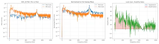
The system

With the theory settled, the design philosophy is simple: anything that needs to be fast and/or deterministic and/or interacts with the physical world is done on the FPGA, anything that doesn’t but still needs to touch the FPGA is done on the hard processor (ARM Cortex-A9), and everything else is done client-side. The system is similar to Linien, albeit much less polished and much more hackable. Hackability here means direct control over as much of the RTL as possible. You can wire the inputs and outputs of basically any two modules together however you want, which makes rapid ad-hoc lab tests easy. So it’s not only a laser-spectroscopy lock, but also a lightweight oscilloscope, spectrum analyzer, PID controller, FIR filter, and function generator, all in one.

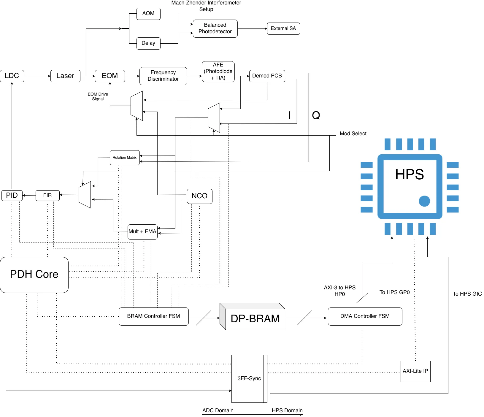
Dotted lines are control/callback signals routed to and from submodules by the PDH core; dashed lines are data taps that can be selected to feed the DMA engine.

TL;DR: it’s a baby Moku.

Protocol timing

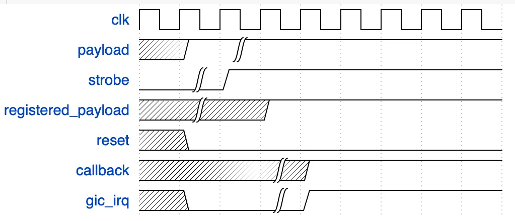
The command word is 32 bits: [31] reset, [30] strobe, [29:26] command code, [25:0] payload. Every transaction has the PS write the word twice, first with strobe low and then with strobe high. The FPGA passes the raw GPIO input through a 3-stage flip-flop synchronizer before decoding it, handling the clock-domain crossing between the PS AXI bus and the 125 MHz fabric clock. A posedge detector on the synchronized strobe fires when that edge comes through, latching the command word and executing it on the same cycle. The callback register is combinatorial off the current state, so it’s valid at that same point, and a 1-cycle interrupt fires coincident with the strobe edge. The C server is blocked on a read() of /dev/uio/pdh_uio, which unblocks when the interrupt fires, and the callback register gets sampled.

CMD_GET_FRAME is different: no interrupt fires on the strobe. The DMA state machine runs its sequence (BRAM fill at the decimated rate, then an AXI4 burst to DDR over HP0), and the interrupt fires when the transfer is done. The server waits on select() with a timeout computed from the decimation depth rather than blocking indefinitely. CMD_IDLE generates no interrupt at all. It just resets the DMA state machine back to armed so the next CMD_GET_FRAME starts clean. The reset bit is completely separate from the strobe path and goes straight to the synchronous reset chain.

PID controller

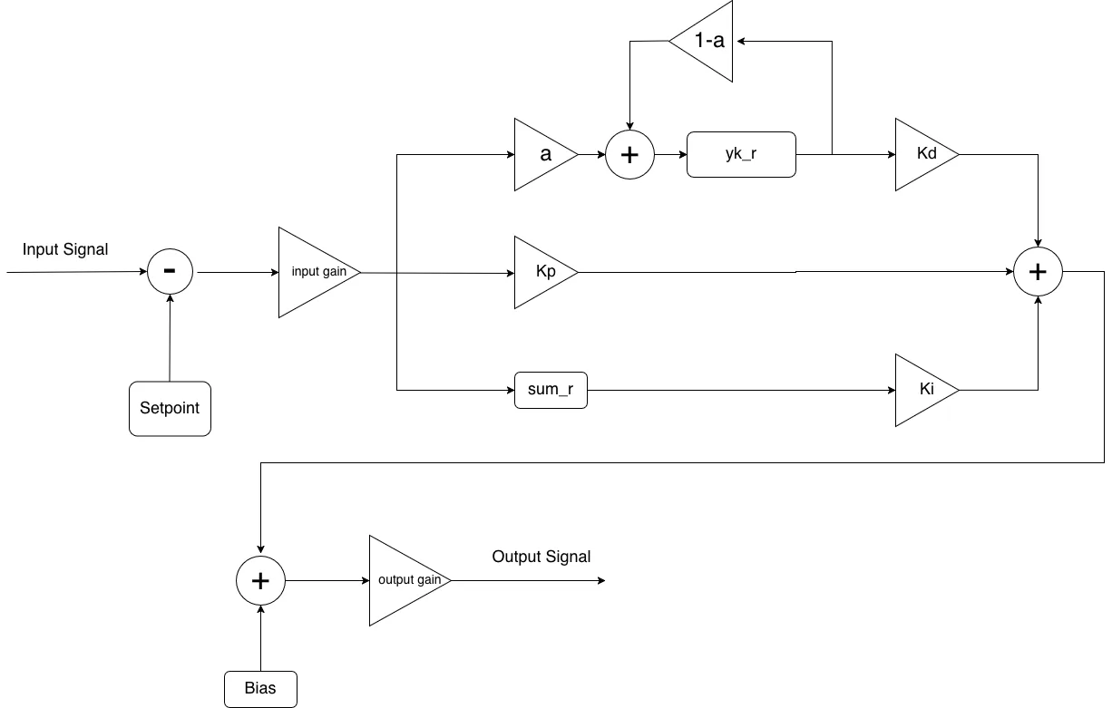
This is the digital realization of the loop filter from the control section. The input has the setpoint subtracted, passes through the input gain stage (egain), and splits into three paths: $K_p$ directly, $K_d$ via the EMA block, and $K_i$ through the running integrator (sum_r). The three products are summed, scaled by the output gain, and then the bias is added.

The derivative path is worth explaining since it isn’t a standard differentiator. The core keeps a running exponential moving average of the error (yk_r), and $K_d$ multiplies the difference between the current error and that average. That difference is the deviation of the error from its recent mean, which approximates the derivative without being as noise-sensitive as a true differentiator; the alpha parameter sets the EMA time constant. The integrator saturates at $\pm 2^{\texttt{satwidth}}$ and freezes in whichever direction would push it further when the output is already railed. Standard anti-windup. Without it the integrator winds up to full scale any time the system is outside the lock pull-in range and then takes forever to recover. The output is 14-bit unsigned offset-binary (DAC code), with 0 V mapped to code 8191, and a decimation parameter slows the PID update rate independently of the NCO, ADC, and DMA, which all keep running at full rate.

TL;DR: standard PID with an EMA derivative and integrator anti-windup. $K_p/K_i/K_d$ are Q15 fractions; the input and output gain stages let you scale without touching the individual terms.

FIR filter

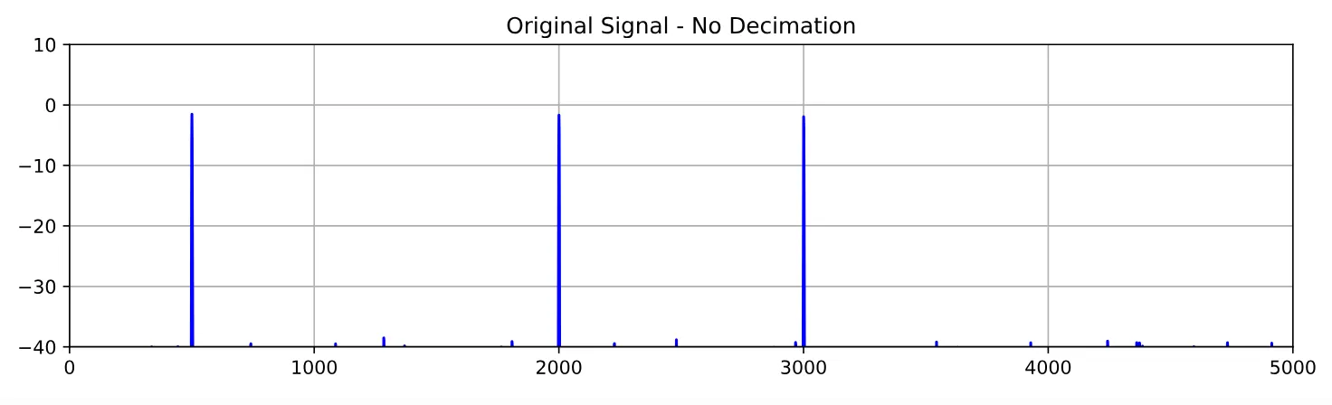
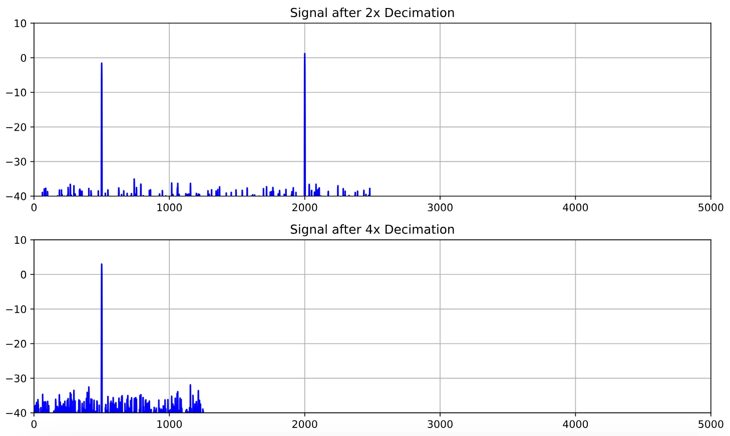
The FIR is there to anti-alias before the PID’s decimation stage.

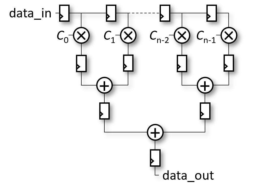
The structure is a 32-tap direct-form filter with a registered saturating adder tree reducing all the tap outputs down to one: the input clocks through a shift register along the top, each stage multiplies by its stored coefficient, the products register, and they get summed pairwise down to the output. Saturation is applied at every add level so overflow can’t propagate up the tree. 32 taps means 5 levels of pairwise adds plus the tap-level register, so 6 cycles of pipeline latency.

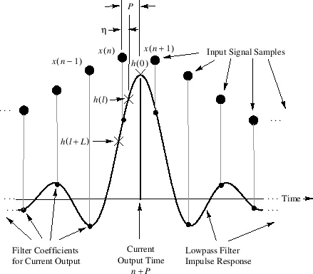
The coefficients are a windowed sinc, the ideal lowpass impulse response truncated to 32 samples and multiplied by a window.

Coefficients are loaded one at a time into a staging memory, then committed to the active tap registers in one atomic shot, so the filter never runs with a partially-updated coefficient set during a live load.

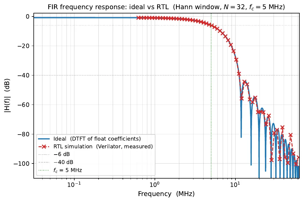
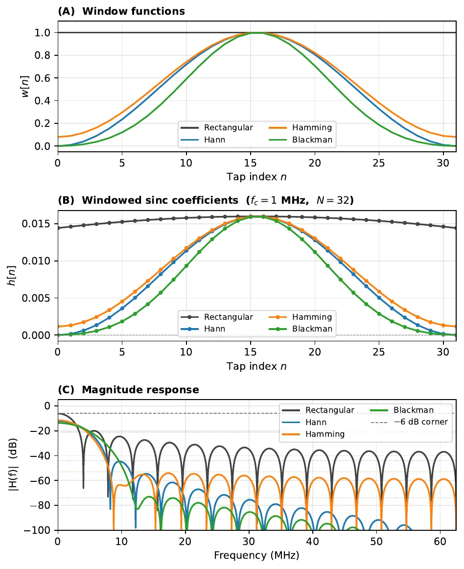
The response on the left is a Hann-windowed design at $f_c = 5$ MHz with $N=32$; the RTL simulation tracks the ideal floating-point response down to about $-80$ dB, roughly where Q15 quantization noise lifts the stopband floor. The right figure shows the window tradeoff: rectangular has the sharpest transition band but terrible sidelobe rejection, while Blackman reaches $-75$ dB or better at the cost of a wider transition. For a PDH lock, where the EOM modulation frequency is well separated from the cavity linewidth, Blackman or Hann is the right call.

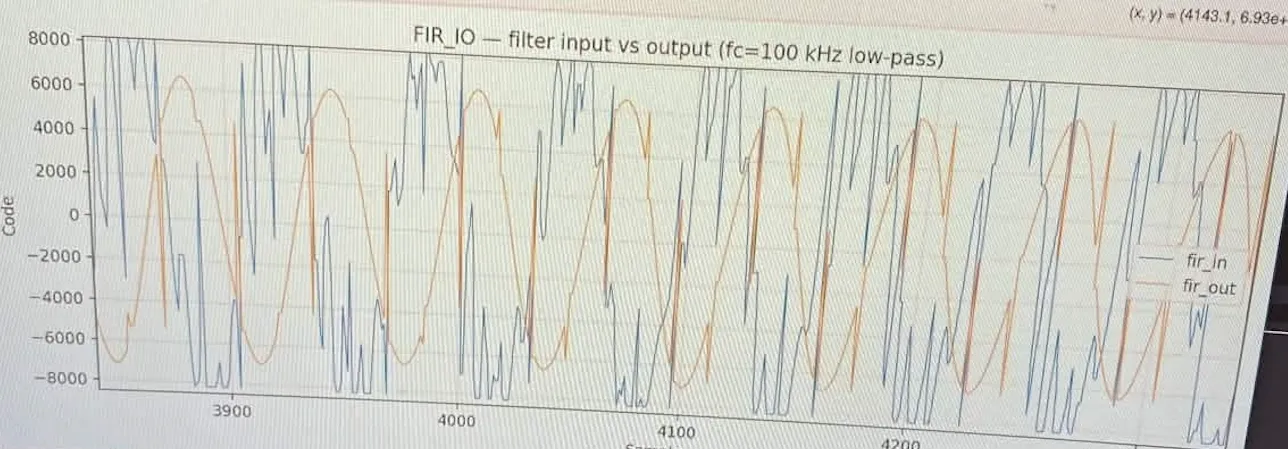
The capture above is from hardware: fir_in is the raw wideband signal going into the filter and fir_out is the 100 kHz lowpass output.

Hardware specifics

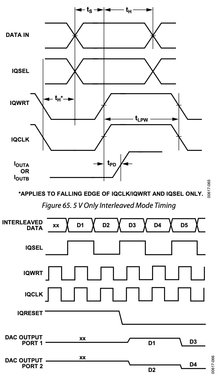
The system currently targets a STEMlab 125-14 (both generations should work, but it’s been tested on Gen1). If porting to another board, make sure the ADC and DAC coding schemes are adjusted accordingly. The AD9767 only has one input port connected on the 125-14, so the system runs it in interleaved mode coherent with the timing below.

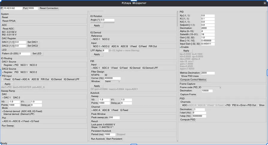
The code is on GitHub.